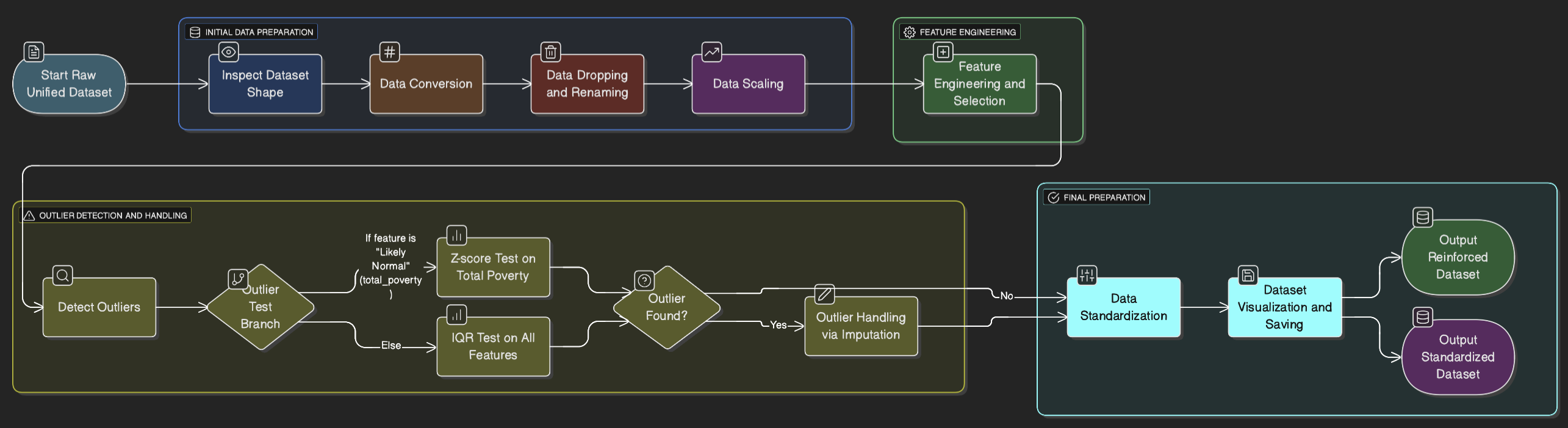
With the data preprocessed and ready, we can now analyze the data to uncover patterns and insights regarding the relationship between poverty, employment, and crime rates across Philippine regions. For now, let's answer our research questions! For a more detailed explanation, proceed to our GitHub repository, specifically the data_analysis.ipynb!
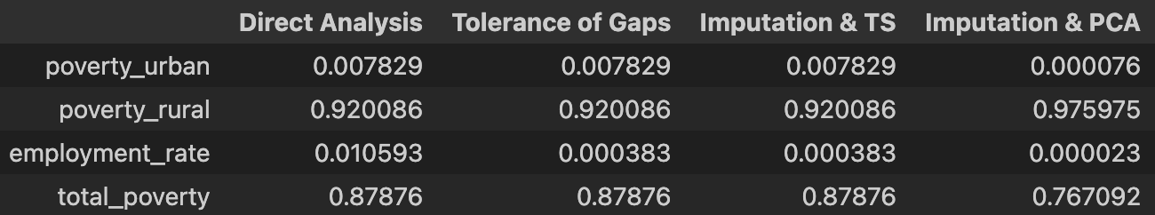
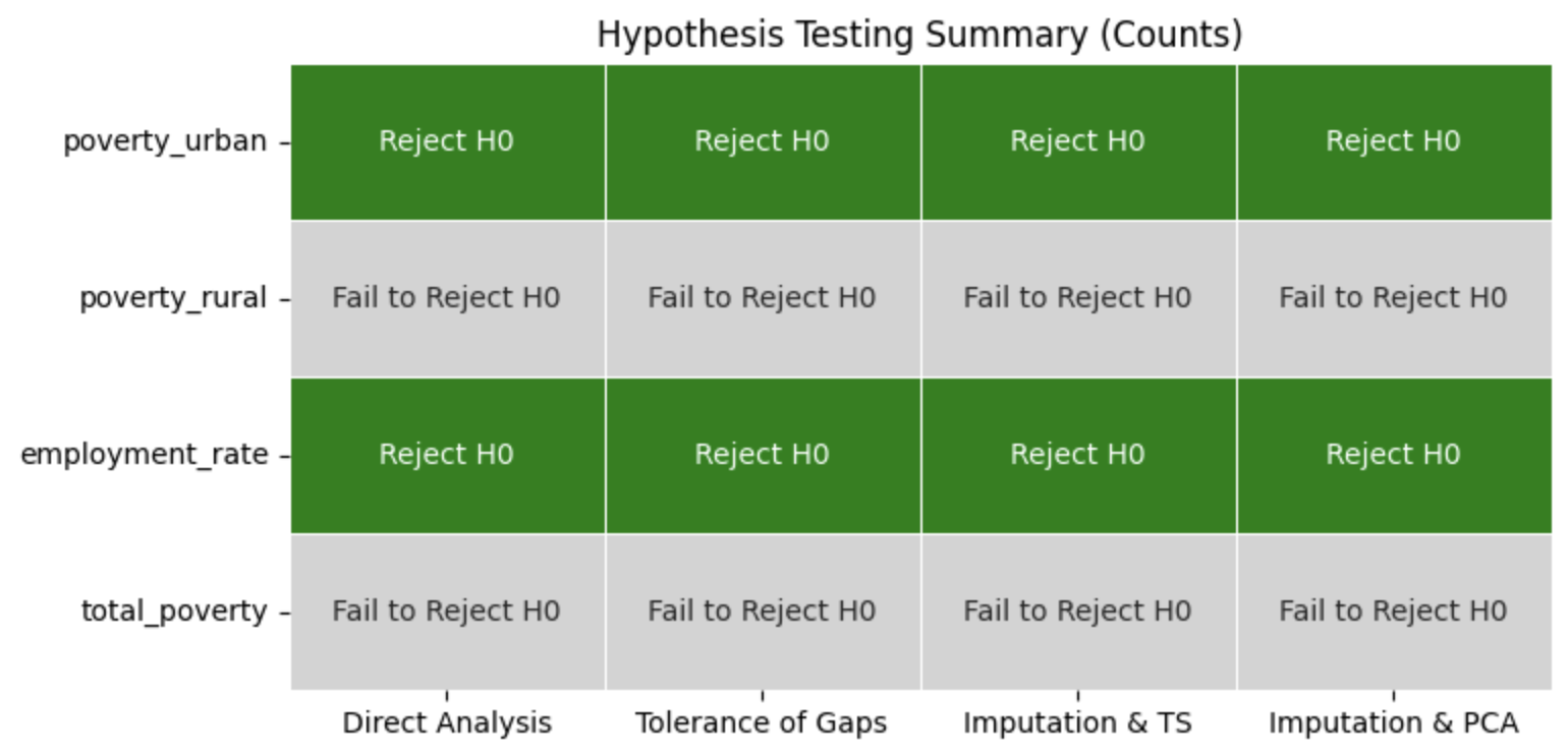
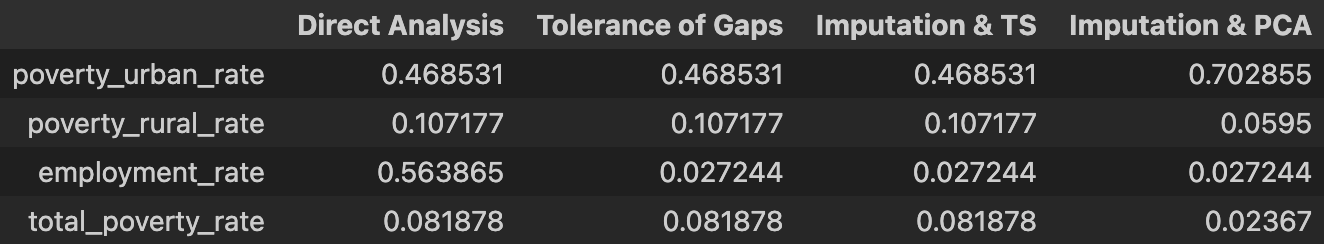
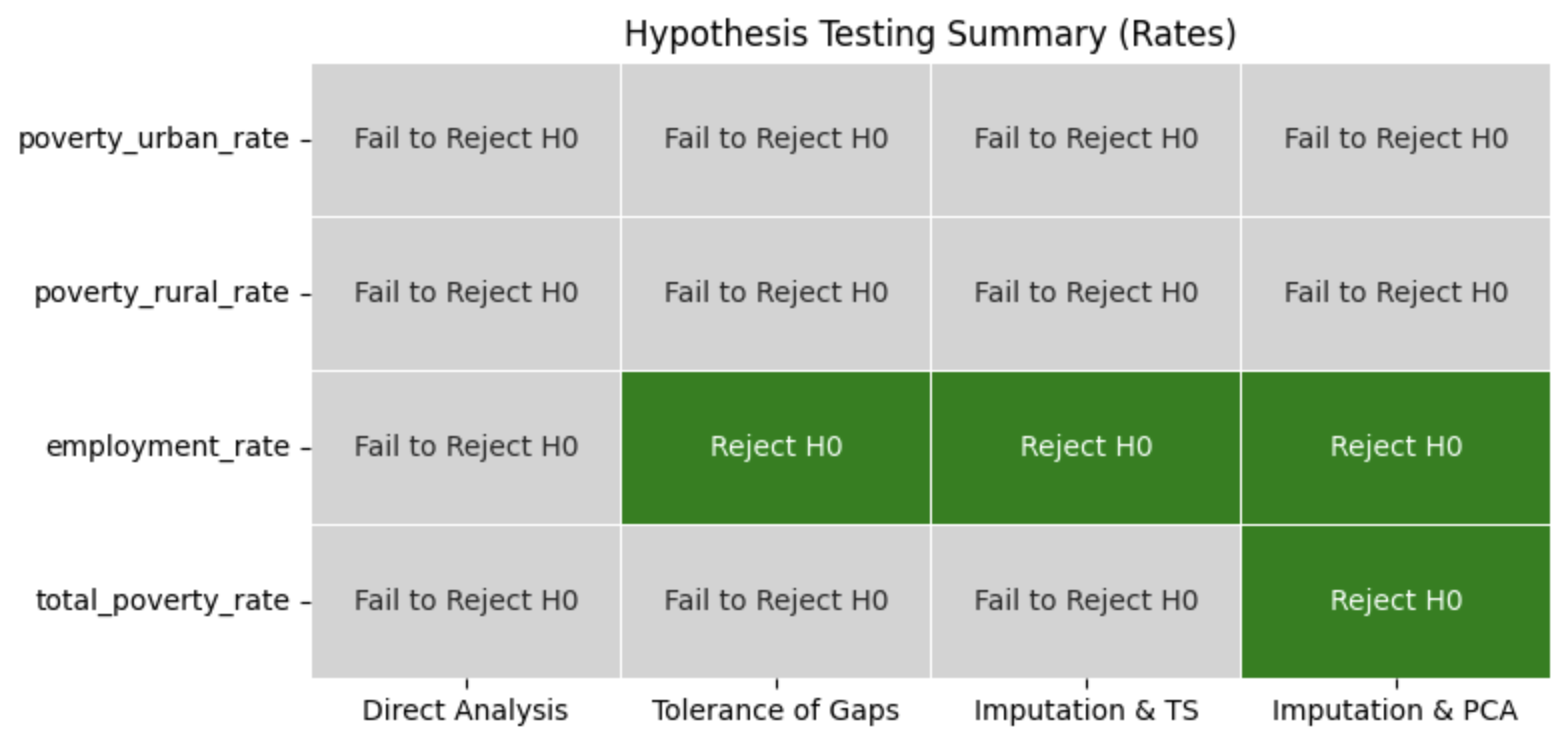
Before explaining the answers to the research questions, do note that we tried four (4) (initially three (3) but due to uniform recommendations and subpar results... we opted to add another one) different approaches to determine and look for possible trends and correlations to properly answer the research questions. Direct Analysis, Tolerance of Gaps, Imputation and Time Series Forecasting, and Imputation + Principal Component Analysis (PCA) were the four (4) analyzed approaches. Each approach gave insights on the available data, and the last method, Imputation + PCA, served to be the most insightful for the answers. Learn more about the approaches done in our GitHub Repository.
1.) What is the correlation between poverty and employment with crime counts/rates across regions in the Philippines?
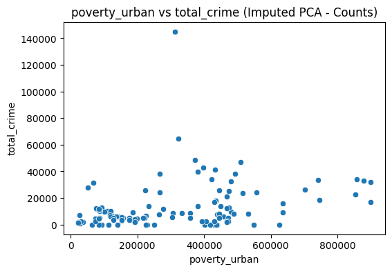
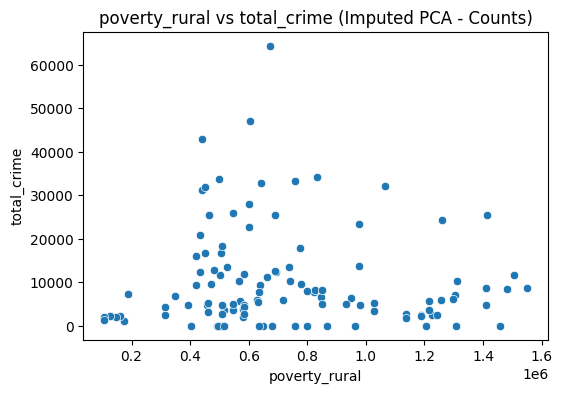
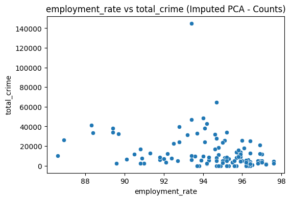
Scatter plots were done to visualize the relationships of poverty and employment with crime. We compared urban poverty, rural poverty, and employment rate to total crime.
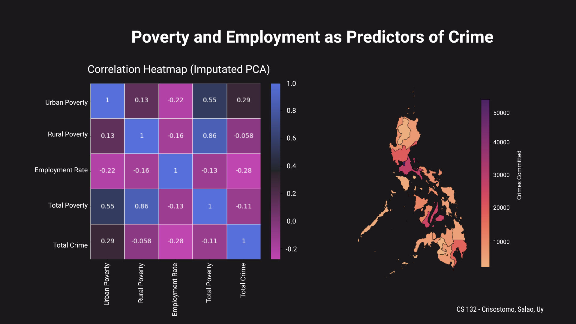
Using these data plots, there is no obvious pattern or trend among the collection of points. Urban-Crime seems to show a slowly rising trend with the more urban population having more crimes committed. The Rural-Crime graph shows a bit of random points, and the same goes for the Employment-Crime graph. A deeper analysis must be done in order to determine the underlying trends that is not so clear to the naked eye. A correlation heatmap is done to visualize and numericize the correlations.
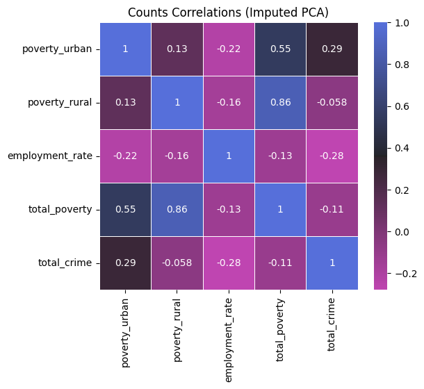
Analyzing this correlation heatmap, it seems that urban poverty (poverty_urban) has the greatest correlation among the other variables with respect to the total crimes (total_crime) committed in a region. Then, employment rate (employment_rate) takes the second indicator; although, note that it shows a negative correlation. Finally, rural poverty (poverty_rural) lastly follows, showing a very close to zero (0) (i.e., absent) correlation to crime.
There could be many reasons for this, such as a more "relaxed" life in rural areas or provinces and other cultural reasons. For now, we will keep it as is. This is not a worry as this observed relationship and reasoning will be further discussed in the successive findings.
Nevertheless, this correlation heatmap directly answers research question number 1 (RQ1). Now, let us look at a more "regional" perspective and point of view.
2.) How do regional variations in these socioeconomic and institutional factors (i.e., poverty and employment) influence differences in crime rates?
Here, we would like to analyze the regional variations or in other words, compare the values in each region. We would mainly use the Imputation and Time Series Forecasting approach for this research question.
First, we will show the time series plots and compare the regions.
From these graphs, we can see that the regions generally follow the same trends.
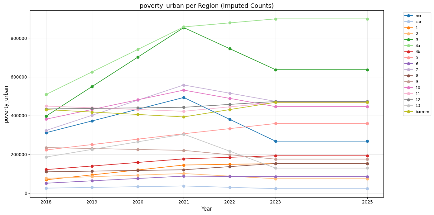
Urban poverty rose from 2018 to 2021 possibly due to the pandemic, and some regions started to recover after the peak in 2021 and declined back through 2022 to 2025.
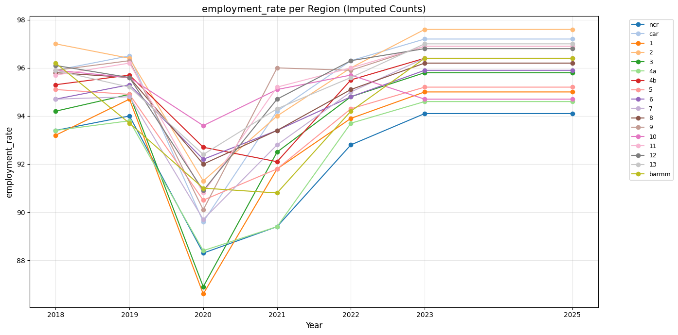
Employment rate also took a huge drop in 2020 possibly due to the pandemic, but it rose back the following year in 2021 and continued to rise or remain stagnant until 2025.
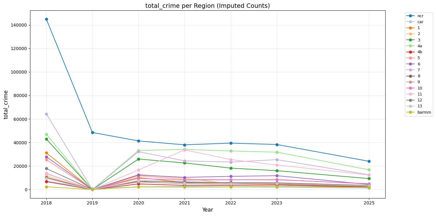
The total crime per region all have a declining trend from 2018 to 2025.
There does not seem to be much of an outlier except for NCR, which was affirmed in the IQR test in the EDA, approximately having 140,000 total number of crimes during 2018.
Looking at the urban poverty of the regions and comparing their total number of crimes, we can see a slight correlation or pattern concerning the region.
Specifically, observing the top five (5) regions in the urban poverty category namely, region 4A, region 3, region 7, region 10, and 12, all of them except region 10 and 12 are also found in the top five (5) number of total crimes committed, but with a slight difference in order.
NCR has the most, followed by region 4A, region 7, region 3, and lastly, region 11. As explained earlier, there is a slight correlation amongst the number of urban poverty and total number of crime, and this holds true for the top five (5) regions.
Moving on to employment rates, all regions do not differ much from each other. Taking the bottom five (5) regions in employment rate, we get NCR, region 4A, region 1, region 3, and region 5.
Out of the five (5) regions, only three (3) of them are in the top five (5) of the total number of crimes, and only two (2) are also part of the top five (5) in urban poverty.
Moving forward, looking at the opposite side and checking the bottom five (5) regions in the urban poverty category, we get regions CAR, 6, 2, 1, and 8.
Now, for the employment rate (highest), we get regions, 2, 9, 11, 13, 12, and for total crime (lowest), we get BARMM, CAR, region 4B, 13, 9.
From here, we can see that CAR (poverty), and region 9 and 13 (employment rate) are both found in the total crime.
Region 4B is the 6th least number of people classified under urban poverty and region 13 ranked 6th. Likewise, region 9 ranked 7th least, which shows a bit of a relationship to the low crimes.
However, BARMM, having the least number of crimes committed, actually ranks high in the urban poverty, ranking at 7th, and ranking 4th in rural poverty, and 6th lowest employment rate.
Despite these counterintuitive placements, they rank the lowest number of crimes. This could be due to many factors such as religion and the 2014 peace deal ending the war in the region and the continuous seek to end conflicts.
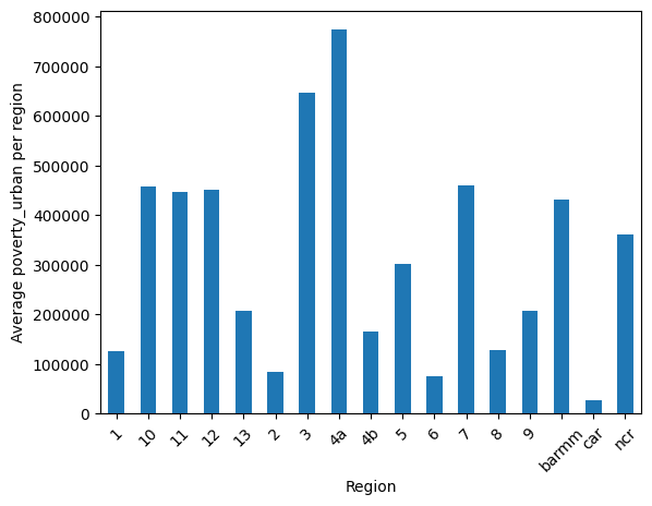
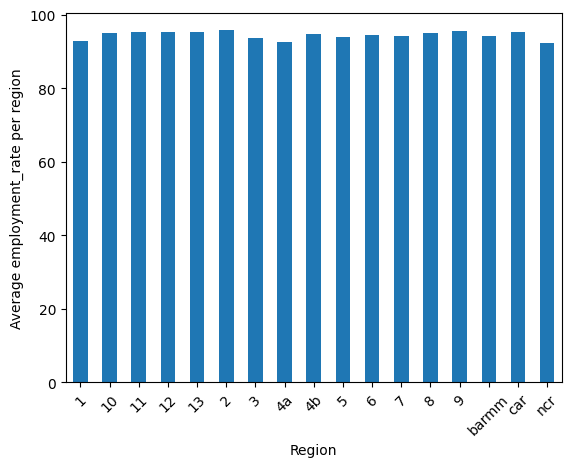
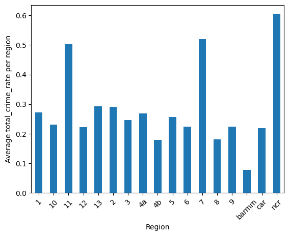
Awesome! Now, let's look at the averages throughout the years in a bar graph to compare them easier.
Here, we can see the average crime rate seem to be higher in three (3) regions, namely NCR, Region 7 (Central Visayas), and Region 11 (Davao Region). There seems to be some relation on the location of a region with crime, which can be due to employment and poverty rates associated to the said locations.
One thing to notice about this "Big 3" is that they are also relatively high on the urban poverty category in their respective regions, which can support the correlation found in RQ1.
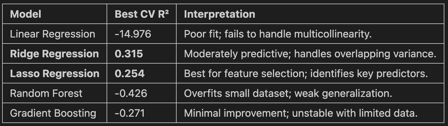
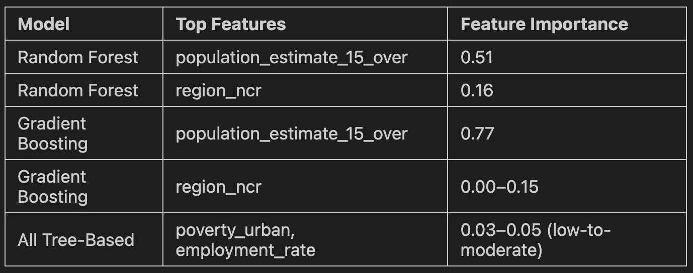
Stay tuned though as it will be shown in the Machine Learning Model section that the NCR region becomes an important feature for tree-based models!
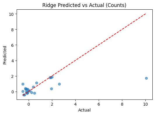
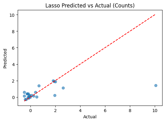
3.) To what extent can improvements in these factors (e.g., reduced poverty, increased employment) predict a decrease in crime rates across regions?
This will be answered using our developed models. Feeling excited? Okay then... proceed to the Machine Learning Model section!